• the theory behind it all
• implementing the thing
• caveats
  • why does ewc work so well?
  • femi, i’ve never even heard of continual learning
• model pruning
• conclusions & meta-lessons

A while ago I replicated the algorithm described by the paper Overcoming catastrophic forgetting in neural networks. I wrote about the process of building understanding around the paper here. I implemented everything in PyTorch in a colab notebook.

The goal of Elastic Weight Consolidation (the main method described in the paper) is to counteract catastrophic fogetting, a phenomena where nerual networks trained on multiple seperate tasks sequentially rapidly forget how to perform old tasks.

(Preventing catastrophic forgetting is an entire sub-field called Continual Learning. The first question that comes to mind is why not just train on old task data? This is called Rehersal and the sub-sub-field of Rehersal-Free CL is concerned with techniques that don’t rely on old data. When I say CL throught this post, assume I’m refering to Rehersal-Free CL.)

Elastic weight consolidation prevents this by figuring out which weights are important for a task, and which weights can be changed and penalizing the model for changeing these weights.

the theory behind it all

The method is as follows. We are given a dataset \( \mathcal{D} \) which we split into two parts, \( \mathcal{D}_A \) and \( \mathcal{D}_B \). We’ve just finished training \( \boldsymbol{\theta}_A \) on dataset \( \mathcal{D}_A \) and now we want to train on dataset \( \mathcal{D}_B \).

Kirkpatrick et al. turn to bayes rule next.

\[ P(\boldsymbol{\theta} | \mathcal{D}) = \frac{P( \mathcal{D} | \boldsymbol{\theta} )P(\boldsymbol{\theta})}{P(\mathcal{D})} \tag{1} \]

What this statement is telling us is that the probablity of any set of paramters \( \boldsymbol{\theta} \) is dependant on three things. The likelihood \( P(\mathcal{D} | \boldsymbol{\theta}) \), the marginal probablity \( P(\mathcal{D}) \), and the prior probablity \( P(\boldsymbol{\theta}) \). We want the set of parameters theta that is most likely under dataset \( \mathcal{D} \).

To make the remaining calculations simpler, let’s take the log of our equation and negate it.

\[ -\ln P(\boldsymbol{\theta} | \mathcal{D}) \propto -\ln P(\mathcal{D} | \boldsymbol{\theta}) - \ln P(\boldsymbol{\theta}) \tag{2} \]

You’ll notice I dropped the marginal probablity. That’s because we have no control over it, and it doesn’t matter when we’re maximizing the probablity of \( \boldsymbol{\theta} \).

The key trick of EWC is that the authors split the dataset, on the left hand side. The equation then becomes.

\[ -\ln P(\boldsymbol{\theta} | \mathcal{D}) \propto -\ln P(\mathcal{D}_B | \boldsymbol{\theta}) - \ln P(\boldsymbol{\theta} | \mathcal{D}_A) \tag{3} \label{loglike} \]

The first term, \( -\ln P(\mathcal{D}_B | \boldsymbol{\theta}) \), is known as the negative log-likelihood. Calculating this is standard practice and nothing new.

The second term is impossible to calculate.

In order to approximate it, we have to understand really what it means. The second term on the left hand side of equation \( \eqref{loglike} \) is equivalent to the loss function of \( \mathcal{D}_A \), \( \mathcal{L}_A(\boldsymbol{\theta}) \). The paper builds on the work of A Practical Bayesian Framework for Backpropagation Networks and uses the 2nd order taylor expansion to approximate \( \mathcal{L}_A(\boldsymbol{\theta}) \) around the already trained, well perfoming¹ model \( \boldsymbol{\theta}^*_A \).

\[ \frac{1}{2}(\boldsymbol{\theta} - \boldsymbol{\theta}^*_A)^T\boldsymbol{F}(\boldsymbol{\theta} - \boldsymbol{\theta}^*_A ) \tag{4} \label{approx} \]

Equation \( \eqref{approx} \) is the said approximation. \( \boldsymbol{F} = \nabla \nabla \mathcal{L}_A(\boldsymbol{\theta}) \)² and is also known as the Observed Fisher Information Matrix. The FIM is calculated right as we finish training on the first task, the old model weights stored, and the old data is discarded.

However, neural networks have a large amount of paramters. Even a model with a 100,000 paramters (very small by modern standards) would need a FIM of size \( 10^{10} \)!!! It’s not even feasible to think about calculating it for larger models.

So the authors get clever. They use the diagonal of the FIM to approximate the real thing. If we let \( \boldsymbol{F}_i \) represent the \( i \)th element on the diagonal of the FIM. Then the final loss function becomes

\[ \mathcal{L}_B(\boldsymbol{\theta}) + \sum_i \frac{\lambda}{2} \boldsymbol{F}_i ( \theta_i - \theta^*_{A,i} )^2 \tag{5} \label{finloas} \]

implementing the thing

Before we talk about actual implementation, we should talk about the “tasks” we use to evaluate the method.

Within the continual learning community, it’s common to use permuted MNIST to benchmark continual learning methods. In permuted MNIST, each task is a permuation. When learning a task, the input to the model is the MNIST data, permuted according to the task’s permutation.

EWC needs two things, it needs the old paramters from the old task, and it needs a calculated FIM.

The first componenet was easy, I could use pytorch’s model.state_dict() function to save and load old paramters. The FIM was a little more tricky.

My first instinct was to just calculate the Hessian and save the diagonal. This was obiviously a bad idea and made more complicated by the fact that pytorch’s backpropagation engine would freak out if i wanted anything higher order than the gradient. After a couple of hours of pulling my hair out, I realize that the authors explicitly say that the FIM can be calculated from first order derivatives. This is (apparently), true! Wikipeida even says so!³ According to these sources, the diagonal of the FIM is \( (\nabla_{\boldsymbol{\theta}} \mathcal{L}_A) ^ 2 \)!

The model I used was a simple MLP with two hidden layers of size 400. I used SGD with momentum and a learning rate of \( 10^{-3} \).

The first thing I wanted to do was see catastrophic forgetting. Here’s a graph showing how performance fares without EWC!

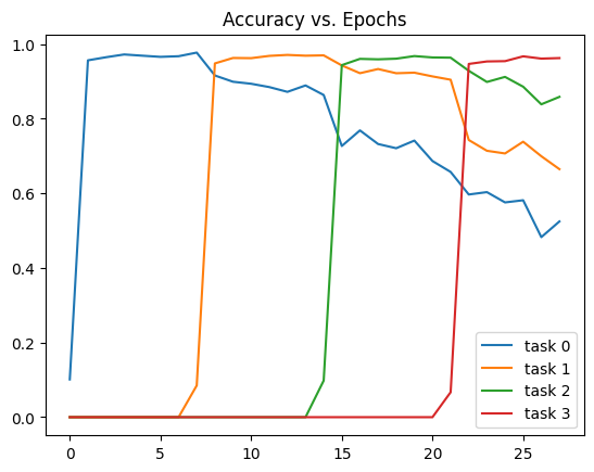
We see model performance decline almost monotonically. After the fourth task, the model is down to 50% accuracy. 50% doesn’t sound too bad, however the MNIST is so easy for this model that it can recieve almost 100% test accuracy after just 1 epoch. Additionally, the model could theortically retain it’s accuracy if it learned to unpermute the inputs at an earlier layer.

Before I show you how the model performs when trained with EWC, i’ll use a different baseline, the \( L_2 \) distance from the old parameters.⁴

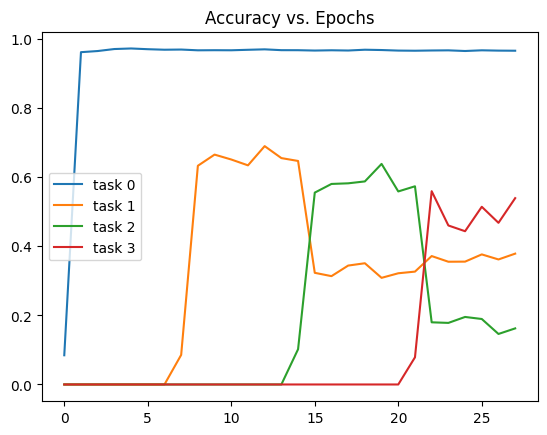
Catastrophic forgetting is prevented at the cost of performance on future tasks.⁵ Not good enough! EWC is much more successful.

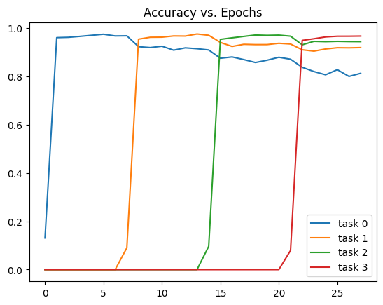
This is drastically better than both prior curves! The model retains above 80% accuracy on all tasks! This seems to be a miracle! Why isn’t EWC more popular?!

caveats

Firstly, I just want to say equation \( \eqref{loglike} \) is wrong. Bayes rule does not allow you to split the conditional like this. The correct form would be⁶

\[ -\ln P(\boldsymbol{\theta} | \mathcal{D}) = -\ln P(\boldsymbol{\theta} | \mathcal{D}_A) - \ln P(\boldsymbol{\theta} | \mathcal{D}_B) \label{correctloglike} \tag{6} \]

This is a very subtle difference, but one that caused me a great headache when reading this paper.

Next, the paper layers approximation upon approximation. Using the 2nd order taylor expansion of the loss function? A (good) approximation. Using the Fisher Information Matrix to approximate the Hessian needed for the 2nd order expansion? An (excellent) approximation. Using the Observed Fisher Information Matrix to approximate the actual Fisher Information Matrix? Another (very good) approximation. However, even after all that approximating, we still take a (this time really bad) final approximation of the FIM as a diagonal matrix. In fact the paper they cite for the idea of using the FIM explicitly warns that the diagonal of the FIM isn’t good enough!

It is important, for the success of this Bayesian method, that the off-diagonal terms of the Hessian should be evaluated. Denker et al.’s method can do this without any additional complexity. The diagonal approximation is no good because of the strong posterior correlations in the parameters.

“Okay Femi,” I hear you say. “EWC is built on shoddy approximations, whatever. Explain why it works so well?”

why does ewc work so well?

Emprically Singh and Alistarh observed that the FIM is a) a decent local approximation of the loss function, and b) mostly sparse off of the diagonal. That is not to say that the off diagonal terms wouldn’t help considerably – they would. I interpret these finding as, go ahead and use the diagonal if you really have too. It’s better than nothing.

Additionally, permuted MNIST is actually very easy. It’s a domain incremental task meaning that the input distribution might change, but the output distribution won’t. Most methods for continual learning don’t struggle on permuted MNIST.

A much harder task is Split MNIST. Split MNIST doesn’t have \( n! \) possible tasks to generate, however the paper that introduced Split MNIST (Hsu et al., 2018) argues that Split MNIST is more representative of tasks we might encounter in the real world. After training one just one more task than I trained on in my replication, the authors report EWC has an average global accuracy (accross all tasks) of 58.85%…

Compare this to the ~90% global accurcay we had on permuted MNIST. So in conclusion, …it kind of doesn’t work.

femi, i’ve never even heard of continual learning

Yeah, and for good reason. For larger models, one might argue it doesn’t matter (see Blessings of Scale). These models are so large and are pre-trained on so much data that they truly do not need continual learning. In fact, continual learning doesn’t need continual learning!

Naive Rehersal (just mixing in old training data) beats out every single continual learning technique we have!⁷ One might argue that the whole field of continual learning is beyond useless. It’s a collection of researchers working with their hands tied behind their backs and making progress there. I would agree for the most part.

model pruning

Don’t get me wrong, CL techniques cannot work at a large scale, but they admit a useful application, model pruning. The (diagonal) Fisher Information Matrix allows you to (roughly) see which parameters are are important to performance, and which ones less so.

We can use this to prune the original network. Lets go with the definition of \( F \) used in \( \eqref{finloas} \). Define \( F_{max} \) as the largest element in \( F \) and \( F_{min} \) as the smallest. We can set a threshold \( T \) such that

\[ T = k(F_{max} - F_{min}) + F_{min} \]

Where \( k \) is some pruning constant on the interval \( [0, 1] \). All weights with a corresponding FIM value that falls below \( T \) are set to zero.

Measure performance of the pruned model as the relative accucuracy when compared to the base model. Formally,

\[ \textrm{Performance} = \frac{\textrm{Pruned Model Accuracy}}{\textrm{Base Model Accuracy}} \].

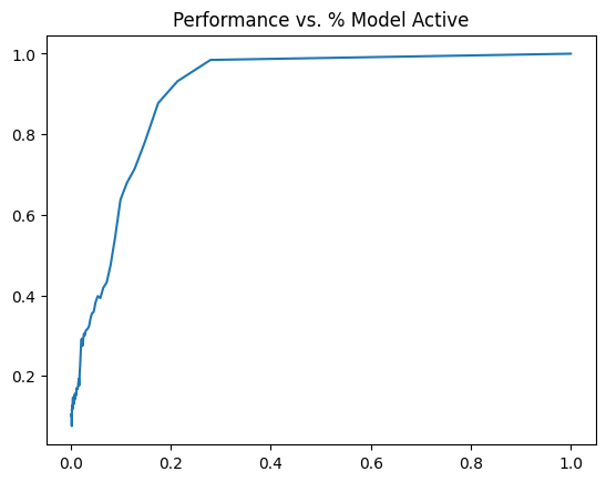
From the above graph, we see that the model maintains pretty much perfect performance until ~30% activity. This is crazy to me! With only 30% of the weights we get most of the performance back. To go a little further we can visualize which weights are active and which weight aren’t.

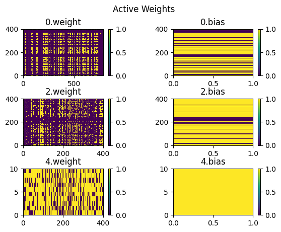
Above is the sparsity graph of the model when ~20% of the weights are non-zero and 92% percent of performance is acheived. The first thing that sticks out is the strong importance fo the biases and the last weight vector. The first two weight matricies are incredibly sparse, and sparse in a strange way.

We see these horizontal and vertical banding that happens across the network. It’s my personal theory that this is caused by blank space in the input image. The model doesn’t really need to read data at these points, thus the weights become redundant.

conclusions & meta-lessons

So to recap, EWC prevents models from forgetting how to perform well on old data by quadratically approximating the loss on said old data around a minimum. This is of limited use for continual learning, but interesting for model pruning.

Was it worth it to replicate this paper? On the whole, I’d say yes! I learned a ton of math on the way and got a few ideas for further interpretability reserach using model pruning! That being said, continual learning won’t take us to AGI, it’s usefulness in smaller models on limited tasks does not make up for the fact that it’s utterly useless for larger models. But it has yet to be investigated as a tool for MLP interpretability. I enjoyed doing this replication, and I hope you enjoyed reading it.

---