I recently spent the better part of last week doing exactly what the title says.

I implemented a 1 layer Feed Foward Network and trained it on (some of) MNIST. All in scratch.

It would help a lot to understand the basics of Deep Learning when reading this, but I’ll try to make it accessible to anyone with a high level understanding of the field.

before coding

the data

MNIST is an image classification dataset consisting of labeled 28 by 28 grayscale images of digits from 0-9. The goal of the model is to correctly identify the label of each image.

example of an MNIST image

For each image, the model should output a series of probablities, representing how likely the model believes that the image belongs to a given class.

For the above image the model might output a vector like

\[ \begin{bmatrix} 0.01 \\ 0.02 \\ 0.01 \\ 0.01 \\ 0.01 \\ 0.08 \\ 0.01 \\ 0.83 \\ 0.01 \\ 0.01 \end{bmatrix} \]

The sum of these entries is one, meaning that it’s a valid probablity distribtuion, and the most likely value is the 8th entry – which corresponds to the number 7.

Our model works purely with vectors and matricies, so we can flatten this 28 by 28 grid into a vector of dimension 784. To make things a little simpler, we can batch inputs to get a matrix of dimension \( 784 \times N \). Where \( N \) is the number of images in the matrix. Our output will then have the shape \( 10 \times N \).

the model

I started by writing out the model formally. Given some inputs \( X \) (\( X \in \mathbb{R}^{784 \times N} \)) our model \( f(X) \) is

\[ H_{1} = W_{1}X + \boldsymbol{b}_1 \]

\[ H_{2} = \textrm{ReLU}(H_1) \]

\[ H_{3} = W_{2}H_{2} + \boldsymbol{b}_2 \]

\[ f(X) = \textrm{Softmax}(H_3) \]

Note that \( W_1 \in \mathbb{R}^{128 \times 784}, \boldsymbol{b}_1 \in \mathbb{R}^{128} \) this means that in the first equation, I add a vector to a matrix. In these cases I broadcast the vector across across the batch dimension of the matrix. The same is true for the second equation.

The columns of \( H_3 \) aren’t guaranteed to sum to one. So the Softmax function normalizes them and ensures that each column is a valid probablity distribution.

Together, all these equations make up what’s called the forward pass, and is one half of the computation we’ll need to do.

scratch, the programming langauge

Scratch is pretty limited.

The main thing we’ll need are multi-dimensional lists of numbers. While scratch does have lists, they’re restricted to one dimension, and can only hold up to 200k elements at a time. This is bad news, as neural networks need a lot of data, and the training set for MNIST contains 60k images of size 784! I’ll talk about how I got around this later.

However, scratch contains most of the math operations we’ll need to actually pull this off. In addition to the 4 basic operators, scratch also contains the natural log and the exponential! (What 10 year old needs the natural log?)

Scratch doesn’t have functions, or any sense of scope, so all variables are global. Instead of functions, scratch has 2 options, custom blocks and messages. List names can not be passed as variables to custom blocks, so I use messages to implement everything.

Messages are signals to various parts of the program. They singal for a block of code to start, but don’t pass along any additional information. I rely on globally avalible buffers and careful reuse of variables to make the most of the messaging system.

coding

init

While we can initalize the bias vectors at 0, the weights need to be initalized carefully to avoid vanishing/exploding gradients. The most common initalization is the xaivier initalization. In the xaiver init, the values of the weights are sampled from a normal distribution with variance

\[ \frac{2}{D_{in} + D_{out}} \]

The only random variable scratch gives us access to is a uniformly distributed one. However, we can create a standard normal with two unifrom variables using the box-muller transform.

\[ \mathcal{N}(0, 1) = \sqrt{-2 \ln U_1} \cos(U_2) \]

Where \( U_1 \in [0, 1] \) and \( U_2 \in [0, 2\pi] \). Finally, we scale by the square root of our target variance.

To store these weights, I create a new scratch list for each one (w_one, w_two) along with the bias vectors (b_one, b_two). I store the input dimensions and the output dimensions in the global variables w_[n]_in_features and w_[n]_out_features.

the code used to initalize one weight matrix.

Notice, that the second random variable, \( U_2 \) is over \( [0, 360] \) instead of \( [0, 2\pi] \). Because of course, scratch operates in degrees.

matrix multiplication

To implement matrix multiplication, I needed three things. 1. A way to treat 1D lists as 2D, 2. Some way to initate the operation, and 3. A place to store the result of the operation.

Storing matricies as 1D lists under the hood actually isn’t anything new, and is how pytorch implements it’s tensors. We can define a simple mapping from two coordinates to 1.

\[ n_{rows} * r + c \]

Where \( r \) and \( c \) are the current row and column of the matrix respectivly, assuming that the matrix is 0-indexed.

Well, this assumption is wrong actually! Scratch lists are 1 indexed, which was an intense source of frustration at the start, but was remedied by pretending everything was 0-indexed and then adding 1 at the end.

With regards to initating the operation, I’ll use the messages I described before. List names cannot be passed as variables, so each matrix multiplication gets it’s own message of the form [first]_[second]_matmul.

the code for one matrix multiplication

The drawback of not having reusable functions is that it’s 10x easier for me to make a mistake. So after each matmul implementation, I immidately compare it to a multiplication I perform by hand.

If you look at the code above, you’ll notice I store the result in a list called the hidden buffer. This list’s only purpose is to store the resulting multiplication. Every multiplication has an output buffer, and you’ll see why I don’t just get rid of them right after I’m done using them later.

The bias is implemented similarly, the only diffrence is I add the single column bias to every column in the hidden matrix.

ReLU stands for Rectified Linear Unit and is what gives the model it’s expressive capablities. It works elementwise implementing the following function on some matrix \( M \)

\[ \textrm{ReLU}(M)_{i, j} = \max(0, M_{i, j}) \]

logsumexp

The final layer is the softmax of every column in the matrix \( H_3 \). Defined as

\[ \textrm{Softmax}(H_3)_{i, j} = \frac{e^{H^3_{i, j}}}{\sum_k e^{H^3_{k, j}}} \]

Like I said earlier, it’s the probablity that the \( j \)th image is the number \( i - 1 \).

The loss – a number which tells us how good the models predictions are – is defined as follows

\[ -\frac{1}{N} \sum^N_{i=1} \ln \textrm{Softmax}(H_3)_{y_i, i} \]

Where \( \boldsymbol{y} \) is a vector in \( \mathbb{R}^N \) that tells us which classes are correct for a given set of images. This defines the Cross Entropy Loss, and our goal is to minimize it.

Now the denomanator of the softmax calculation is tricky to calculate. For numerical stablity reasons, we don’t calculate it directly. Instead, we perform a little trick described here. Below is the code I wrote (dragged?) to implement this.

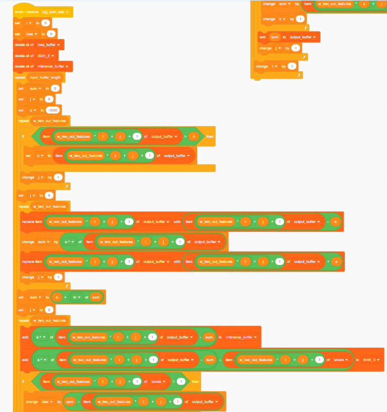
It’s beautiful.

the backward pass

Fortunatly, the backward pass uses much of the same operations that the foward pass does. The only exception being the Heavyside function, which I’ll describe later.

At a high level, Gradient Descent works by finding the direction that loss decreases the most and making a small step in that direction. To find this direction, we find the gradient with repsect to the loss of all four of the trainable parameters.

The main way to do this is via the chain rule. We can’t directly calculate the derivative of the loss wrt to any one parameter, but we can do so indirectly.

For example, to calculate \( \frac{dL}{d W_2} \) we calculate

\[ \frac{dL}{dW_2} = \frac{dL}{dH_3} \frac{dH_3}{dW_2} \]

Computing gradients like this is called the backward pass, and is the other half of the computation I mentioned earlier.

This is true for scalar functions with scalar outputs, but each of these things are matricies and that complicates things. You can’t just multiply two matrices together.

For this, I asked ChatGPT.

I felt fine asking ChatGPT about the details for three reasons

1. Nothing I’m doing isn’t standard, and has probably been done before. In fact, ChatGPT was able to pick up on the fact that I was creating a NN given only the equations.

2. If I were to ever do this again in a real programming language, I wouldn’t touch matrix based backprop with a 10ft pole. Andrej Kaparthy has a good tutorial on implementing scalar valued backprop that doesn’t give me an aynurism.

3. It made the progamming (dragging?) 10 times faster. This project easily could’ve taken a month if I had to teach my self the details to matrix calculus to make this.

That being said, you’ll see why this might have been an issue later.

Anyways, here’s the graidents for each parameter matrix according to ChatGPT

\[ \frac{dL}{d\boldsymbol{b}_1} = (W_2^T(f(X) - Y) \odot \textrm{Heaviside}(H_1)) \] \[ \frac{dL}{dW_1} = (W_2^T(f(X) - Y) \odot \textrm{Heaviside}(H_1))X^T \] \[ \frac{dL}{d\boldsymbol{b}_2} = f(X) - Y \] \[ \frac{dL}{dW_2} = (f(X) - Y)H_2^T \]

You’ll notice a lot of reused computation here, it’s something I took advantage of to make implementing this less of a nightmare. Note that Y is the labels matrix. \( Y \in \mathbb{R}^{10 \times N} \), it has \( N \) columns each containing a one hot encoded label of each image.

The Heaviside function is the derivative of the ReLU function, and is defined as follows

\[ \textrm{Heaviside}(X)_{i, j} = \begin{cases} 1 & X_{i, j} \geq 0 \\ 0 & X_{i, j} < 0 \end{cases} \]

Now all that’s left to do is implement the fucntions, load in the data, and profit right?

then it all went horribly wrong

You see, I’ve been spoiled by pytorch. I’ve never really had to think about how the arrays were stored under pytorch’s hood. Yes I knew they were flat arrays for fast indexing, but in what order. Even though I had checked each matmul by had, I hadn’t bothered to check the order of each array. When I say order, I mean the order the values exist in memory.

There are two major orders, column major and row major. I was assuming everything was column major, but outputting the results of my matrix multiplications in row major order! Neural Networks fail silently, and it wasn’t until my loss inital loss started trending up that I realized I would have to rewrite everything I had done so far. By now, I’d call myself a seinor scratch developer, so reimplementing everything only took a day.

image from the craft of coding

To test everything, I created some dummy datapoints and had the model overfit to them. The results were beautiful. Loss, quickly and rapidly decreasing.

loss curve on 2 random datapoints

MNIST, was less beautiful.

loading in the data

MNIST, despite being small by modern standards, is massive by scratch standards. It isn’t possible to load the entire dataset into the input buffer, nor did I have the energy left to write a batch loader for a toy project. So I loaded in 250 datapoints and tried to make due with that.

The model is small, and our dataset is smaller. Neural Networks are not known for being sample efficent, and I am using no forms of regularization. I’m using full batch gradient descent and train on 200 steps for each graph here.

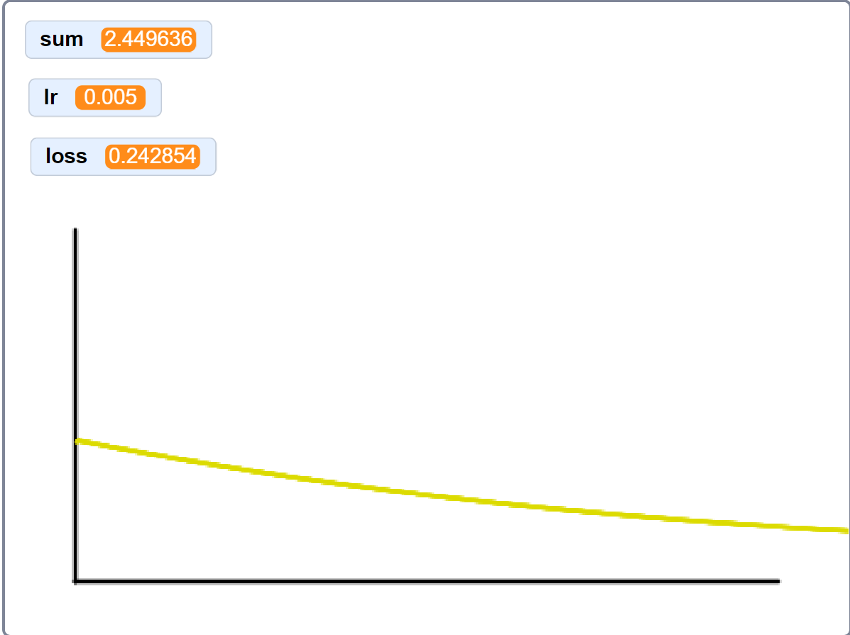
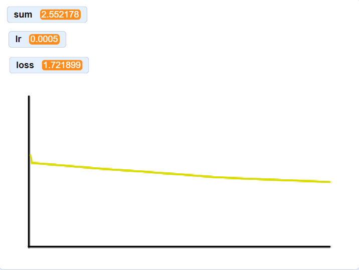
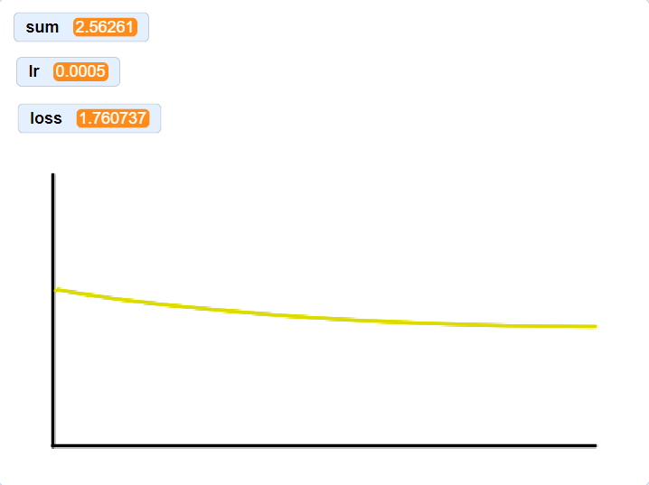
The graphs below are a result of using progressively larger subsets of the 250 samples. I didn’t have matplotlib, so please excuse the janky plotting setup. Loss starts at ~2.3 for each graph. Notice that I decreased the learning rate by an order of magintude compared to the plot above, this is because I was suffering from the Dying ReLU problem. The heaviside function stops gradient flow through zeroed out neruons, in some cases, this completely causes those neruons to never fire again. While I could implement a new activation function, decreasing the learning rate seemed to work.

loss curve on one MNIST sample

loss curve on four MNIST samples

loss curve on sixteen MNIST samples

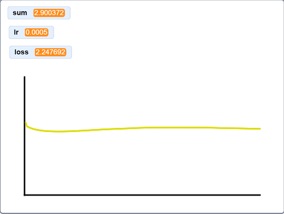loss curve on sixty-four MNIST samples

Training on 64 samples took 5+ hours on my machine, all for this depressing ass loss graph, so I didn’t bother training on the full subset.

So can you build a nerual network in scratch? Yes! Will it work? Well…

looking back

Why did it really fail to converge. Was it because of shoddy GPT math? Possibly. However, the model has everything pretty much stacked against it.

• Training is unbearably slow (in the time I might do 5 training steps on 250 samples, I could’ve finished 5 epochs on the full 60k images in the equivilant pytorch implementation) as a result even the 4 sample graph took around 15 mintues of training.
• Data is incredilbly limited, even sample efficent models trained on MNIST need a few thousand examples.
• The model is pretty small, and super shallow. While yes, I could’ve added more hidden layers. I also have spent a week+ on this.
• The loss curve was smooth! I suspect this is because I’m not using SGD, but I wasn’t expecting it to be this smooth, what’s up with that?

But this whole ordeal taught me a valuable lesson in paitence, and made me appricate pytorch so much more. Feel free to look at the code and try to find any bugs! I’ve removed the MNIST data because scratch wouldn’t let me publish a project so large, but here’s the code I used to generate the image and label files.

import numpy as np
import pandas as pd
from torchvision import datasets, transforms

# Load the MNIST dataset
transform = transforms.Compose([transforms.ToTensor()])
mnist_dataset = datasets.MNIST(root='./data', train=True, download=True, transform=transform)

# Prepare the data for the first 250 samples
images = []
labels = []

for i in range(250):
    image, label = mnist_dataset[i]
    # Flatten the image and add it to the images list
    flattened_image = image.view(-1).numpy()
    images.append(flattened_image)
    
    # Create a one-hot encoded label
    one_hot_label = np.zeros(10)
    one_hot_label[label] = 1
    labels.append(one_hot_label)

# Convert lists to numpy arrays
images = np.array(images).reshape(-1, 1)  # Column-major order
labels = np.array(labels).reshape(-1, 1)  # Column-major order

# Convert numpy arrays to pandas DataFrames
images_df = pd.DataFrame(images)
labels_df = pd.DataFrame(labels)

# Save DataFrames to CSV files
images_df.to_csv('images.csv', header=False, index=False)
labels_df.to_csv('labels.csv', header=False, index=False)

onward to the next project.