I recently spent a couple months working on a research project. The goal was to submit to NeurIPS’ new High School track. I’d never done something like this, and I learned a lot about doing ML research by trying.

I’ll split this post into two parts. This part will be more technical, describing the results. I really don’t feel like writing another research paper about this, so this blog post will have to do.

The next part will be about the journey, describing small tricks and meta-skills I learned about doing ML research. I think that post will be helpful if you’re like I was, young and excited to try research.

Introduction

The theme of NIPS’ HS track was something like “ML for social good”, asking that we write a paper applying ML to some socital problem. A couple of friends of mine had recently been working on a seizure prediction project, so we decided to try adapting that.

The main problem that seizure prediction is trying to solve is that around 20-40% of people with epilepsy have refactory epilepsy. Meaning, drugs don’t work well to treat them. There are many options for treatment, but seizure prediction aims to improve the quality of life of the afflicted, by at least telling them in advance that a seizure will occur. This way, they can receive preemptive treatment or get somewhere safe to have the seizure.

The main way seizures are predicted is under what I’ll call the Standard Framework (SF). Under the SF, seizure prediction takes electroencephalogram (EEG) data and uses machine learning to predict if a seizure will happen in a window of time specified by two numbers. The Seizure Prediction Horizon (SPH) and the Seizure Occurance Period (SOP).

When we make a prediction, we’re saying that within SOP minutes, but not before SPH minutes, a seizure will occur. These two numbers are hyper parameters, and are fixed before training. This makes seizure prediction under the SF a classification problem.

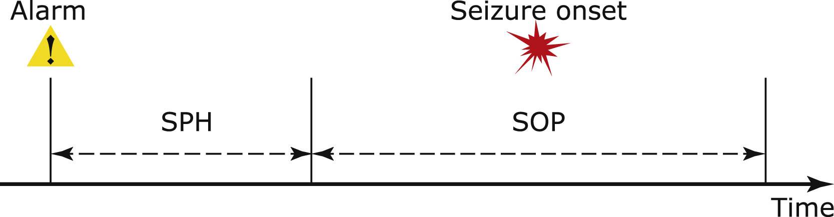Example from Troung et al.

Research has suggested that there is no optimal SPH/SOP for all people.¹ Instead, these numbers vary from paitent to paitent.

In this work, I propose the Epileptic Uncertainty Framework (EUF). In the EUF we keep the SOP, but redefine it as the Maximum Prediction Horizon (MPH). Additonally, we predict a distribution over possibile times that the seizure will occur. Making seizure prediction under the EUF a classification and regression problem.

I acheive similar classification results to prior work, and very calibrated regression distributions, as seen by brier score. By training the model to predict a distribution, we go from being able to answer the question, “What is the probablity I will have a seizure in this specific time window not set by me” to being able to answer, “What is the probablity I’ll have a seizure within x minutes”, where x is controlled by the paitent.

Methodology

Dataset

I use the CHBMIT seizure dataset.² The dataset consists of >300 hours of EEG data over 23 patients, with labeled seizure start and end times.

The EEG data has 23 channels and is broken up into multiple files that are around 1 hour long. In between each of the files are gaps that are on average around ~3 seconds long.

I draw samples that are ten minutes long. To extend the use of the dataset, I draw overlapping samples. When a sample crosses over a file gap, I just fill it with zeros. I run a filtering process on the whole dataset to filter out samples that are more than 3% zeros.

The seizure signals are very weak, so I multiply them by $ 10^3 $ and run them through the Short-Time Fourier Transform (STFT). STFT turns the raw signals into spectrograms, which gives the model time and frequency information. In theory, the model can implement it’s own STFT, but I find that you need an extra OOM of parameters to do the job of the STFT.

The end result of that is a large 23 channel image which I resize into a 256 by 256 image. Finally a tensor of shape $ (23, 256, 256) $ is passed to the model.

For data with seizure that happen later than the MPH, the label is set to $ \infty $, otherwise, it’s set for the time between the end of the data and the next seizure. All the non-$\infty$ data is scaled to have variance one (and shifted to have mean 0 in the case of heteroskedastic regression).

I only train on a single patient due to not wanting to work on this project for another week.

Epileptic Uncertainty Framework

Under EUF, the model is represented as a function $ f $ which maps data to distribution parameters. What $ f $ is approximating is the conditional distribution $ p(t | \mathbf{X}) $. In english, “the probablity density of a seizure happening in exactly $ t $ seconds from now given the EEG data”

We assume that the conditional distribution is from a family of distributions $ \mathcal{F} $. Each distribution in this family is uniquely defined by a parameter vector $ \mathbf{\theta} $. So our model will take in the EEG data $ \mathbf{X} $ and return the parameter vector $ \mathbf{\theta} $ specifying the distribution which we’ll use to approximate the conditional distribution.

For this task, we assume that epliepsy is a possion process and model the distribution over the next seizure time as an exponential distribution. The parameter vector is just a single value $\lambda$ and the distribution is

\[ p’(t) = \lambda \exp(-\lambda t) \]

However, to make training easier, we use the MPH to bound how far the model has to predict. So the model actually outputs the vector

\[ \begin{bmatrix} \omega & \mathbf{\theta} \end{bmatrix} \]

$\mathbf{\theta}$ is still the same parameter vector as before, but $\omega$ is the probablity that a seizure happpens in the MPH at all. Phrased mathematically

\[ p(\Omega) = \omega \]

Where $\Omega$ is the event where a seizure occurs within the MPH.

Now, instead of approximating the conditional, we now approximate

\[ p(t | \mathbf{X}, \Omega) \]

In english, “the probability density that a seizure happens in $ t $ seconds given the data and that a seizure occurs within the MPH.”

So the probablity density at $ t $ is

\[ p(t | \mathbf{X}, \Omega)p(\Omega) \]

Model

I use a model very similar in archecture to AlexNet. I adjusted in the nubmer channels that had to pass through the model, and some filter sizing. I also make the model Multi-Head. Meaning for each parameter in the output vector, a seperate set of MLP layers is set to extract different information from the shared layers without interfering with each other.

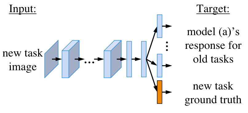Example of Multiple head model from Li and Hoiem.

I find that single head training doesn’t work very well. The model has to struggle to maintain performance on all of the tasks. The classification head is trained seperately from those that describe the conditional distribution.

Training

To train the model, I use the Maximum Likelihood Objective. We’re given a dataset $ \mathcal{D} = {(\mathbf{X}_i, t_i)}_N $ consisting of $ N $ sameples which we assume are independent of each other, but identically distributed.

The likelihood is equal to

\[ \prod_{i=1}^N p’(t | \mathbf{X}, \Omega)p’(\Omega) \]

To make maximizing easier, we move to log space, and, as is tradition, make everything negaitve and switch to minimizing. For the exponential distribution, this means that the optimization criterion $\mathcal{L}$ is

\[ \mathcal{L}(\mathcal{D}) = \sum_{i=1}^N \lambda t_i - \ln \lambda - \ln \omega \]

Out of curiosity, I tried a different distribution. The Normal distribution. There isn’t really a good argument to use this distribution though, I just found interesting results when training. The Normal criterion is

\[ \mathcal{L}_{Normal}(\mathcal{D}) = \sum_{i=1}^N \frac{(\mu - t_i)^2}{\sigma^2} + \frac{\ln 2 \pi \sigma^2}{2} - \ln \omega \]

A major problem when using multiple heads is Catastrophic Forgetting. The performance of one head goes down as the other head goes up. Training changes the shared layers without regard for the other head. To minimize this, I use the regularization provided in the paper Learning Without Forgetting by Li and Hoiem.³

It’s an additional term added to the loss that prevents the predicted distribution of the classification head from moving to far from it’s original state, while still being flexible enough to learn the new task. The loss is simply

\[ D_\textrm{KL}(\omega_{new} || \omega_{old}) \]

In english, “The KL divergence between the distributions predicted by the new and previous model”

Note that is distribution is the classification distribution denoted by $ \omega $. It’s a Boltzmann distribution over 2 states: a seizure will happen within the MPH, or not.

This loss works very well to prevent Catastrophic Forgetting, without any hyperparameter tuning!

When training the regression distribution I only train on positive samples. To prevent the classification head from updating I stop gradient flow from the MLE term of the optimization criterion.

Training the Gaussian Head

When the family of distributions is Gaussian with differing variance, the regression is called heteroskedastic. Training heteroskdastic models can be hard, because of the first term in the loss function. Stirn et al. Identify this in their paper Faithful Heteroskedastic Regression in Nueral Networks⁴ and propose two measures to resolve it.

First, prevent graident flow from the varience head (the $ \sigma^2 $ term) to the shared layers. Next, to remove the influence of the varience head, scale the gradient of the regression head by $ \sigma^2 $ during the backward pass. These two methods are necessary to get acceptable performance on the regression head.

Specific training details can be found in the attached colab notebook.

Results

First, to evaluation classification performance, I use three metrics. AUROC, False Positive Rate per Hour (FPR/H), and Sensitivity. These are standard throught the seizure prediction field.

Next, to evaulate regression performance, I use another three metrics. RMSE, Briar Score, and Negative Log Likelihood (Loss).

For those unfamilar, the Briar Score is a common forcasting metric ranging from 0 to 1. The equation for it is as follows

\[ \textrm{BS} = \frac{1}{N} \sum_{i=1}^N (l_i - p’_i)^2 \]

Where $ l_i $ is 1 if a seizure occurs within a given time interval, and $ p_i’ $ is the probablity predicted of a seizure happening in that interval. A Briar score of 0 indicates perfect calibration, while a Briar Score of 1 indicates the worst possible performance.

To get the time intervals to make predicitons over, I create a range of confidence intervals for the given distribution, then I multiply the confidence level by the probablity predicted by the classification head to get the model’s probablity for a seizure happening there.

I perform 5 fold cross validation with a holdout test set to determine these metrics.

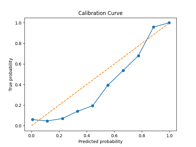
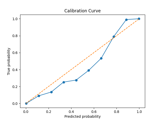
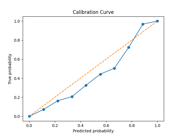
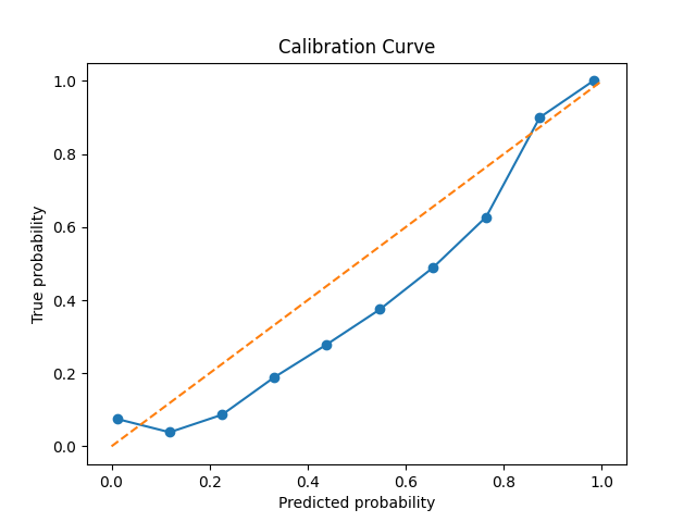
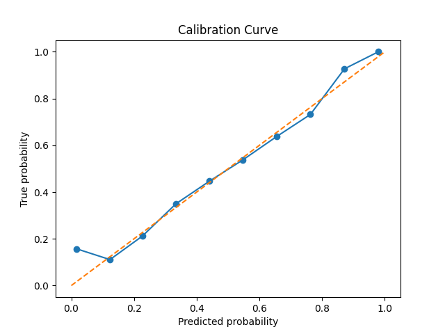
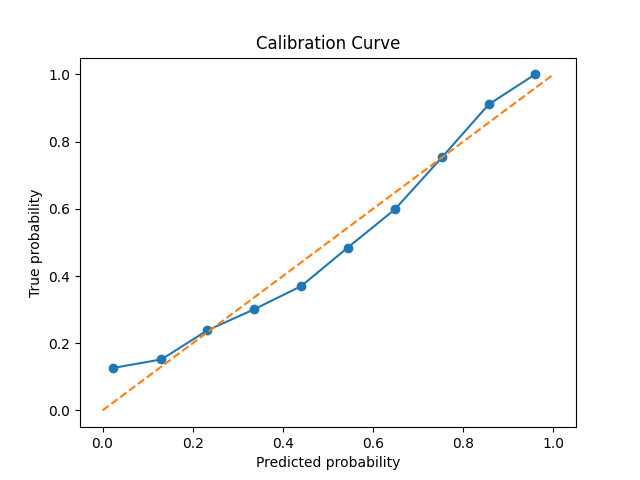
Additionally, I also plot calibration curves. These are a more qualitative way to see if the predictions made by the distribtuion can be trusted and provide an intutive sense of model performance.

Regression type	AUROC ⬆️	FPR/H ⬇️	Sensitivity ⬆️	RMSE ⬇️	Briar ⬇️	Loss ⬇️
Gaussian	$ 0.987 \pm 0.004 $	$ 0.386 \pm 0.090 $	$ 0.955 \pm 0.049 $	$ 0.962 \pm 0.064 $	$ 0.130 \pm 0.020 $	$ 0.150 \pm 0.040 $
Exponential	$ 0.983 \pm 0.007 $	$ 0.462 \pm 0.219 $	$ 0.935 \pm 0.076 $	$ 1.058 \pm 0.174 $	$ 0.141 \pm 0.030 $	$ 1.63 \pm 0.208 $
Turong et al.⁵ (SF)	$ 85.7 \pm 0.000 $	$ 0.24 \pm 0.000 $	N/A	N/A	N/A	N/A
Rasheed et al.⁶ (SF)	N/A	$ 0.05 $	$ 96 $	N/A	N/A	N/A

The arrows indicate whether a lower or higher score is better.

Calibration curves for the Exponential model

Calibration curves for the Gaussian model

These classification results are very similar to the work of Troung et al.⁵ and Rasheed et al.⁶, who also use a similar model archetecture, and acheive results out of our error bars only for FPR/H.

As we see from the calibration curves and briar scores, when the model says that there’s a $ p $ pecent chance of a seizure within their specificed time window, there usually is a $ p $ percent chance, though the model tends towards over-confidence.

Gaussian and Exponential regression don’t differ significantly in their performance. I will note that the Exponential model was much harder to train, and required a little bit of tuning hyper parameters. I didn’t tune much however, so this might explain the weaker performance.

Where the two families do differ though, is their interpretation. The distribution given by the Gaussian is best interpreted as a window of variable length. “There is a $ p $ percent chance that a seizure will take place between times $ a $ and $ b $.” However, there’s no good reason to assume that epilepsy is a Gaussian process.

The interpretation of the Exponential is much more convient. “The probablity that you will have a seizure within $ t $ minutes is $ p $.” This warning time can be adjusted as needed to suit the patient.

Conclusion and Discussion

Despite interesting inital results showing that the EUF is a strong alternative to the SF, there are many limitations to this work.

I only trained on one patient
I did no hyperparameter tuning
The RMSE is oddly close to the varience of the data
CHBMIT data is limited in quantity.
The model is ~80M parameters, and uses 23 channels of seizure data. How can we use a smaller model and train on less channels?

Future directions include

Multi-Patient Pretraining & Paitent Fine-Tuning
EUF without the MPH hyperparameter.
Different model architectures and thier effect on performance.
Model distillation, and few channel prediction on edge devices.

Thank you for reading.

Bandarabadi, Mojtaba, Jalil Rasekhi, César A. Teixeira, Mohammad R. Karami, and António Dourado. “On the Proper Selection of Preictal Period for Seizure Prediction.” Epilepsy & Behavior 46 (May 1, 2015): 158–66. https://doi.org/10.1016/j.yebeh.2015.03.010. ↩
Ali Shoeb. Application of Machine Learning to Epileptic Seizure Onset Detection and Treatment. PhD Thesis, Massachusetts Institute of Technology, September 2009. ↩
Li, Zhizhong, and Derek Hoiem. “Learning without Forgetting.” arXiv, February 14, 2017. https://doi.org/10.48550/arXiv.1606.09282. ↩
Stirn, Andrew, Hans-Hermann Wessels, Megan Schertzer, Laura Pereira, Neville E. Sanjana, and David A. Knowles. “Faithful Heteroscedastic Regression with Neural Networks.” arXiv, December 18, 2022. https://doi.org/10.48550/arXiv.2212.09184. ↩
Truong, Nhan Duy, Anh Duy Nguyen, Levin Kuhlmann, Mohammad Reza Bonyadi, Jiawei Yang, Samuel Ippolito, and Omid Kavehei. “Convolutional Neural Networks for Seizure Prediction Using Intracranial and Scalp Electroencephalogram.” Neural Networks 105 (September 1, 2018): 104–11. https://doi.org/10.1016/j.neunet.2018.04.018. ↩ ↩²
Rasheed, Khansa, Junaid Qadir, Terence J. O’Brien, Levin Kuhlmann, and Adeel Razi. “A Generative Model to Synthesize EEG Data for Epileptic Seizure Prediction.” arXiv, December 1, 2020. http://arxiv.org/abs/2012.00430. ↩ ↩²

« prev home

Regression type	AUROC ⬆️	FPR/H ⬇️	Sensitivity ⬆️	RMSE ⬇️	Briar ⬇️	Loss ⬇️
Gaussian	\( 0.987 \pm 0.004 \)	\( 0.386 \pm 0.090 \)	\( 0.955 \pm 0.049 \)	\( 0.962 \pm 0.064 \)	\( 0.130 \pm 0.020 \)	\( 0.150 \pm 0.040 \)
Exponential	\( 0.983 \pm 0.007 \)	\( 0.462 \pm 0.219 \)	\( 0.935 \pm 0.076 \)	\( 1.058 \pm 0.174 \)	\( 0.141 \pm 0.030 \)	\( 1.63 \pm 0.208 \)
Turong et al.⁵ (SF)	\( 85.7 \pm 0.000 \)	\( 0.24 \pm 0.000 \)	N/A	N/A	N/A	N/A
Rasheed et al.⁶ (SF)	N/A	\( 0.05 \)	\( 96 \)	N/A	N/A	N/A

Epileptic Uncertainty Framework Technical Report